3. Flagging Records Using Associated Information
Source:vignettes/flagging_records.Rmd
flagging_records.RmdIntroduction
Ensuring data quality is a critical step in biodiversity analysis. This vignette demonstrates how to clean occurrence records by identifying and flagging errors derived from record metadata (such as invalid dates, fossils, or cultivated specimens) and spatial artifacts (such as coordinates that fall on capitals, biodiversity institutions, or are geographic outliers).
We will use a combination of RuHere functions for flagging metadata issues and duplicates, and the CoordinateCleaner package for additional spatial tests.
Proposed workflow
The main idea of the package is to provide full control and
reproducibility over the record-removal process. This is achieved by
creating flag columns in the dataset, which are logical
variables indicating whether a record passed a given test
(TRUE) or failed it (FALSE). This approach
allows users to:
- Visuallize and inspect potentially erroneous records interactively before deciding whether to remove them.
- Define exceptions; that is, retain records that were flagged or remove records that were not flagged.
- Save flagged records to separate files, with information indicating why each record was excluded.
- Generate reports summarizing the cleaning process, making it more transparent and reproducible.
Overview of the functions:
-
remove_invalid_coordinates(): removes invalid geographic coordinates. -
flag_fossil(): scans description columns for terms like “fossil” or “paleontological” to avoid mixing modern distribution data with fossil records. -
flag_cultivated(): identifies specimens from botanical gardens, greenhouses, or plantations based on habitat and locality remarks. -
flag_inaturalist(): specifically targets iNaturalist records. By setting research_grade = FALSE, we flag observations that haven’t been peer-verified by the community. -
flag_year(): flags records collected outside a plausible time range or those with missing dates. -
flag_duplicates(): identifies and flags duplicated records. -
remove_flagged(): removes flagged records.
Getting ready
At this stage, you should have an occurrence dataset that has been
standardized using the format_columns() function and merged
with bind_here(). For additional details on this workflow,
see the vignette “1. Obtaining and preparing species occurrence
data”. Ideally, these records should also be standardized for
spatial consistency of country and state information. See the vignette
“2. Ensuring Spatial Consistency” for further
details.
To illustrate how the function works, we use the example occurrence dataset included in the package, which contains records for three species: the Paraná pine (Araucaria angustifolia), the azure jay (Cyanocorax caeruleus), and the yellow trumpet tree (Handroanthus albus).
Removing invalid coordinates
(remove_invalid_coordinates())
Before conducting any spatial validation or modeling, it is essential
to ensure the coordinates are valid. The
remove_invalid_coordinates() function filters out records
where coordinates are non-numeric, missing (NA), or fall
outside the valid global range (Latitude: -90 to 90; Longitude: -180 to
180).
By setting return_invalid = TRUE, the function returns a
list containing both the clean ($valid) and discarded
($invalid) records, which is useful if you want to inspect
the records that were removed. We then update our working dataset
(occ) to keep only the valid records.
# Remove invalid coordinates and store the result as a list to separate valid/invalid data
occ_split <- remove_invalid_coordinates(
  occ = occurrences,
  long = "decimalLongitude",
  lat = "decimalLatitude",
  return_invalid = TRUE
)

# Records with invalid coordinates
occ_split$invalid[, c("species", "decimalLongitude", "decimalLatitude")]
#>                         species decimalLongitude decimalLatitude
#> 376      Araucaria angustifolia               NA              NA
#> 3606       Cyanocorax caeruleus               NA              NA
#> 3768 Handroanthus serratifolius               NA              NA

# Update the main 'occ' data frame to contain only the valid records
occ <- occ_split$valid
Flagging based on metadata information
After ensuring that the coordinates are valid, the next step is to assess the quality of the biological and temporal information associated with each record. Occurrence datasets often contain valuable additional information describing the conditions under which the occurrence was recorded. These additional columns are referred to as metadata.
RuHere provides four specialized functions to identify
common metadata-related issues:
Fossil records
If the goal is to study the contemporary distribution of a species,
fossil records should be excluded. The flag_fossil()
function scans the metadata for terms indicating that a record
corresponds to a fossil.
occ <- flag_fossil(occ) # Scan for fossil-related terms
# Number of records flagged as fossil
sum(!occ$fossil_flag) # No records flagged as fossil
#> [1] 0
Cultivated individuals
For plants, cultivated individuals may represent populations
occurring outside the natural range of the species. The
flag_cultivated() function scans the metadata for terms
indicating that a record corresponds to a cultivated individual. This
function is heavily inspired by the getCult() function from
the plantR package:
occ <- flag_cultivated(occ) # Scan for fossil-related terms
# Number of records flagged as fossil
sum(!occ$cultivated_flag)
#> [1] 14
Records from iNaturalist
Some records, especially in GBIF, are sourced from the citizen
science project iNaturalist.
Because many of these occurrences are recorded by non-specialists, you
may wish to exclude them from your analyses. However, a subset of
iNaturalist records is classified as Research Grade, indicating
a higher level of confidence in the species identification. The
flag_inaturalist() function allows you to flag all
iNaturalist records or only those that are not classified as Research
Grade:
# Flag all iNaturalist records (including Research Grade)
occ_inat <- flag_inaturalist(occ,
                             research_grade = TRUE) #Flag even when is research-grade
sum(!occ_inat$inaturalist_flag) #Number of flagged records
#> [1] 869

# Flag only iNaturalist records without Research Grade
occ <- flag_inaturalist(occ,
                        research_grade = FALSE) # Flags only non-peer-verified iNaturalist records
sum(!occ$inaturalist_flag) #All inaturalist records are classified as Research Grade
#> [1] 0
Records outside a year range
Depending on your objectives, you may wish to exclude records that fall outside a specific temporal range. For example, when fitting ecological niche models using climate variables, very old records may represent populations collected in regions that have since changed and may no longer be suitable for the species. As an example, we flag records collected before 1980:
occ <- flag_year(occ, lower_limit = 1980,
                 upper_limit = NULL) #We could specify a upper limit as well
sum(!occ$year_flag) #Number of flagged records
#> [1] 198
Flagging duplicates
Some records are duplicates, that means, they have the same coordinates. Some of them are full duplicates, that means, additionaly to have the same coordinates, they also have the same metadata.
In the example provided in the package, we have been already removed the duplicated records. But to ilustrate the function, let’s create a new dataset with the records duplicates:
# Duplicated records
new_occ <- rbind(occurrences[1:1000, ], occurrences[1:100,])
RuHere provides several options to deal with duplicates:
- Flag duplicates based only on coordinates: for most cases, you may wish to keep only one record among the duplicated. By default, the kept record is choosen randomly. In RuHere we can control which record will be kept. For example, we can keep the most recent and/or prioritize records from a specific data_source:
# Flag records and keep the most recent and preferably from GBIF:
# Create vector to prioritize gbif records
preferable_datasource <- c("gbif", "specieslink", "idigbio")
occ_dup1 <- flag_duplicates(occ = new_occ, continuous_variable = "year",
                            categorical_variable = "data_source",
                            priority_categories = preferable_datasource)
sum(!occ_dup1$duplicated_flag) #Number of flagged records
#> [1] 100- Flag duplicates based on coordinates and metadata: in some cases, you may wish to consider duplicates only the records that were collected in the same place and also in the same time. That means, records collected in the same place but in different years were not considered duplicates:
# Flag duplicates based on coordinates and year
occ_dup2 <- flag_duplicates(occ = new_occ, additional_groups = "year")- Flag duplicates based on cells of a raster: if you have a SpatRaster, you can consider as duplicates all the records that falls in the same cell.
# Import raster
data("worldclim", package = "RuHere")
wc <- terra::unwrap(worldclim) #Unpack raster
# Flag duplicates based in raster cells and keep the most recent
occ_dup3 <- flag_duplicates(occ = new_occ, continuous_variable = "year",
                            by_cell = TRUE, raster_variable = wc)
If you are working with a large dataset, we recommend flagging and removing duplicate records as a first step after data standardization. More details on how to remove flagged records are provided below.
Spatial cleaning (CoordinateCleaner)
After verifying the metadata, the next step is to address spatial
artifacts. For this stage, we integrate the
CoordinateCleaner package into our workflow. This package
provides a robust set of ready-to-use functions that are fully
compatible with RuHere outputs, allowing for automated
identification of common geographic errors in biodiversity data.
Spatial artifacts often occur when coordinates are assigned to general locations, such as a country’s capital, a state center, or a biodiversity institution, rather than the actual collection site.
Implement flags from CoordinateCleaner
CoordinateCleaner is an R package that performs automated tests to identify suspicious geographic coordinates. Among its various functions, it compares occurrence coordinates against reference databases of country and province centroids, country capitals, urban areas, and biodiversity institutions. For a comprehensive overview of the available methods, see the paper linked here.
RuHere is fully compatible with the flags generated
by CoordinateCleaner, as both packages add logical flag
columns to the dataset (prefixed with .). To apply the
desired coordinate checks, you simply need to use the
clean_coordinates() function:
# Install the package if necessary
# if(!require("CoordinateCleaner")){
#   install.packages("CoordinateCleaner")
# }

# Loading the package
library(CoordinateCleaner)

# Run spatial check using some tests
occ <- clean_coordinates(x = occ,
                         tests = c("capitals", "centroids", "equal",
                                   "institutions", "zeros"))
#> Testing coordinate validity
#> Flagged 0 records.
#> Testing equal lat/lon
#> Flagged 3 records.
#> Testing zero coordinates
#> Flagged 6 records.
#> Testing country capitals
#> Flagged 23 records.
#> Testing country centroids
#> Flagged 7 records.
#> Testing biodiversity institutions
#> Flagged 6 records.
#> Flagged 39 of 4077 records, EQ = 0.01.
The final columns of the occurrence dataset contain the results of the CoordinateCleaner validation. The summary column only reports whether a record passed all applied tests, and can be ignored for the purposes of this vignette.
head(occ[,19:25])
#>   .val .equ .zer .cap .cen .inst .summary
#> 1 TRUE TRUE TRUE TRUE TRUE  TRUE     TRUE
#> 2 TRUE TRUE TRUE TRUE TRUE  TRUE     TRUE
#> 3 TRUE TRUE TRUE TRUE TRUE  TRUE     TRUE
#> 4 TRUE TRUE TRUE TRUE TRUE  TRUE     TRUE
#> 5 TRUE TRUE TRUE TRUE TRUE  TRUE     TRUE
#> 6 TRUE TRUE TRUE TRUE TRUE  TRUE     TRUE
Map of occurrence flags
Once records have been flagged, it is highly recommended to visualize them to assess whether the flagging is accurate before proceeding with final record removal.
RuHere provides two options for mapping flagged records: an
interactive option via map_here(), which uses the
mapview package, and a static option via
ggmap_here(), which uses ggplot2. Let’s see
the flagged record of the Paraná Pine:
Note: In this vignette, the map generated with
map_here()is a static snapshot of the interactive map produced in RStudio.
# Interactive map with map_here()
map_here(occ, species = "Araucaria angustifolia", label = "record_id", cex = 4)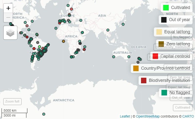
# Static map with ggplot
ggmap_here(occ, species = "Araucaria angustifolia",
           show_no_flagged = FALSE) # Do not show unflagged records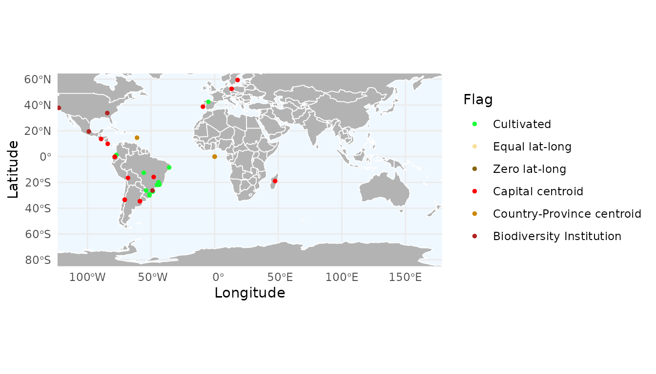
With ggmap_here(), we can also plot each flag in a
separate panel by setting facet_wrap = TRUE:
ggmap_here(occ, species = "Araucaria angustifolia",
           facet_wrap = TRUE)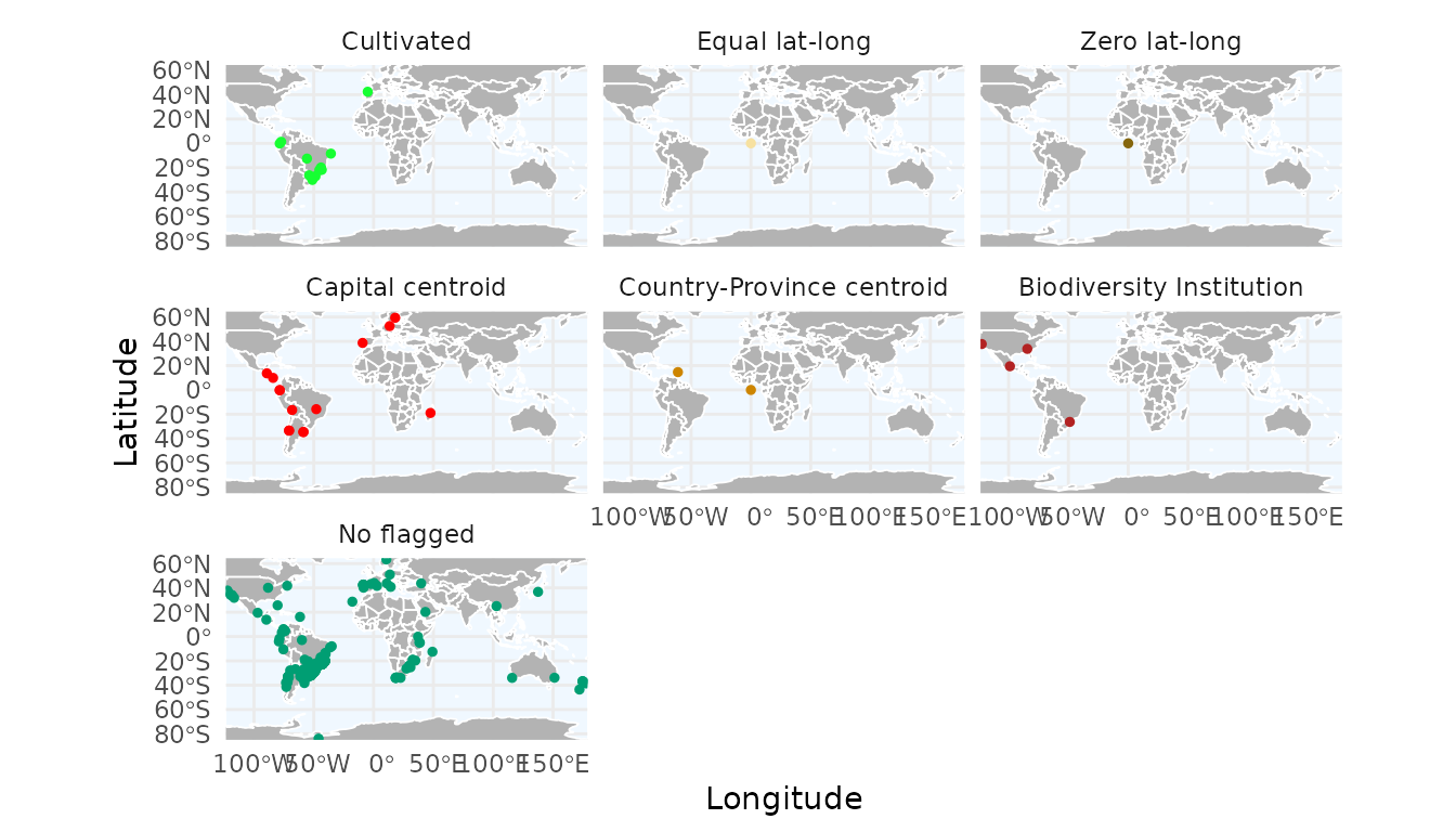
Get consensus across multiple flags
We can obtain a consensus across multiple flags. The consensus can be computed in two ways:
- A record is considered valid (
TRUE) only if all specified flags are valid (TRUE). - A record is considered valid (
TRUE) if at least one specified flag is valid (TRUE).
As an example, we compute a consensus using the cultivated
and year flags. In this case, cultivated records are flagged as
invalid only if they were also collected before 1980. By default, the
function creates a new column named "consensus_flag", but a
custom name can be provided. Here, we name the new flag as
"old_cultivated".
occ_consensus <- flag_consensus(occ,
                                flags = c("cultivated", "year"),
                                consensus_rule = "any_true",
                                flag_name = "old_cultivated")

# Records flagged because they are cultivated and collected before 1980
occ_consensus_flagged <- occ_consensus[!occ_consensus$old_cultivated, ]
occ_consensus_flagged[, c("species", "cultivated_flag", "year_flag", "old_cultivated")]
#>                         species cultivated_flag year_flag old_cultivated
#> 1381     Araucaria angustifolia           FALSE     FALSE          FALSE
#> 1388     Araucaria angustifolia           FALSE     FALSE          FALSE
#> 1424     Araucaria angustifolia           FALSE     FALSE          FALSE
#> 4769 Handroanthus serratifolius           FALSE     FALSE          FALSE
We can visualize this custom flag using map_here() or
ggmap_here(). Because it is a user-defined flag, it must be
specified via the additional_flags and
names_additional_flags arguments, and a color must also be
provided for plotting:
ggmap_here(occ_consensus,
           flags = c("year", "cultivated"),            # Specific flags to show
           additional_flags = "old_cultivated",        # Column name of the custom flag
           names_additional_flags = "Old & cultivated",# Label used in the legend
           col_additional_flags = "red",                # Color for the custom flag
           show_no_flagged = FALSE)                      # Do not show unflagged records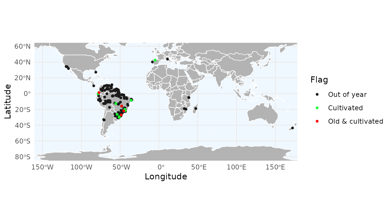
Removing flagged records
After flagging potential issues, we can use the
remove_flagged() function to clean the dataset. This
function is highly flexible, allowing you to filter records based on the
flags generated and also apply manual overrides using the
force_keep and force_remove arguments:
force_keep: a vector of record IDs that you want to keep in the dataset, even if they were flagged as FALSE by one of the functions.force_remove: a vector of record IDs that you want to exclude, even if they passed all automated tests (flagged as TRUE).
As an example, suppose that the records "gbif_17175" and
"gbif_6108" are known, valid herbarium specimens that were
mistakenly flagged as cultivated, while "gbif_5516" and
"specieslink_1091" are records you know to be incorrect but
were not captured by any automated flag.
We can also specify a directory in which to save the removed records. In this example, we use a temporary directory, but in practice you should define a permanent location:
# Create directory to save removed records
path_to_save <- file.path(tempdir(), "removed_records")
dir.create(path_to_save)

# Identify records to force keeping and removing
to_keep <- c("gbif_17175", "gbif_6108")
to_remove <- c("gbif_5516", "specieslink_1091")

# Remove flagged records with manual control
# and save removed records to a folder
occ_cleaned <- remove_flagged(occ = occ,
                              flags = "all",
                              column_id = "record_id",
                              force_keep = to_keep,
                              force_remove = to_remove,
                              save_flagged = TRUE,
                              output_dir = path_to_save)

# Total number of records
nrow(occ)
#> [1] 4077
# Number of valid records
nrow(occ_cleaned)
#> [1] 3837
# Number of records removed
nrow(occ) - nrow(occ_cleaned)
#> [1] 240
We can inspect the directory specified in path_to_save
to see the files containing the removed records. By default, the files
are saved in GZIP format, which is a compressed format that can be read
using data.table::fread().
fs::dir_tree(path_to_save)
#> Temp/removed_records
#> ├── Biodiversity Institution.gz
#> ├── Capital centroid.gz
#> ├── Country-Province centroid.gz
#> ├── Cultivated.gz
#> ├── Equal lat-long.gz
#> └── Zero lat-long.gz
This approach provides a simple and transparent way to maintain control over the cleaning process, allowing you to incorporate your expert knowledge as researcher to complement automated data-quality checks.
Summarizing flags
After flagging the records, we can create a bar plot summarizing the number of records flagged by each flagging function:
flag_summary <- summarize_flags(occ)The function returns a data.frame summarizing the number
of records per flag and a ggplot2 object displaying this
summary as a bar plot:
# Data.frame summarizing the number of records per flag
flag_summary$df_summary
#>                         Flag    n
#> 6             Equal lat-long    3
#> 7              Zero lat-long    6
#> 10  Biodiversity Institution    6
#> 9  Country-Province centroid    7
#> 1                 Cultivated   14
#> 8           Capital centroid   23
#> 4                Out of year  198
#> 11                     Valid 3837
# Bar plot
flag_summary$plot_summary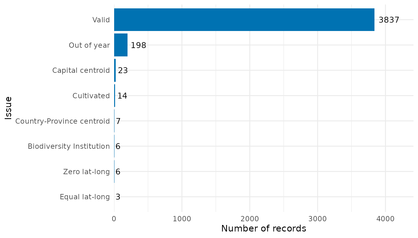
The function can also read flagged occurrence data that were saved
when records were removed. To do so, simply specify the same directory
used in remove_flagged():
# Summarize removed records using saved data
flag_summary_dir <- summarize_flags(flagged_dir = path_to_save,
                                    show_unflagged = FALSE, # Do not show unflagged records
                                    fill = "firebrick") # Change color of bars
flag_summary_dir$plot_summary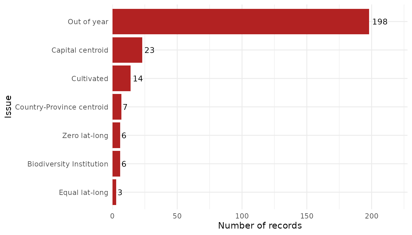
Since the output is a ggplot2 object, it can be saved
using ggplot2::ggsave():
ggplot2::ggsave(filename = file.path(path_to_save, "Summary.png"),
                plot = flag_summary_dir$plot_summary, width = 8, height = 5,
                dpi = 600)
Spatial aggregation of records and flags
While visualizing individual points is useful for specific inspections, aggregating data into spatial grids helps identify broad geographic patterns, such as “hotspots” of record density or regions with high concentrations of data quality issues.
Mapping species richness and record density
By default, richness_here() calculates the number of
unique species per cell. You can also calculate the total number of
records to identify sampling effort. The granularity of the grid is
controlled by the res argument, which defines the spatial
resolution in decimal degrees.
# Create a grid of species richness
r_richness <- richness_here(occ, summary = "species", res = 2)

# Create a grid of record density (total number of occurrences)
r_records <- richness_here(occ, summary = "records", res = 2)

# Plotting the results
ggrid_here(r_richness)
ggrid_here(r_records)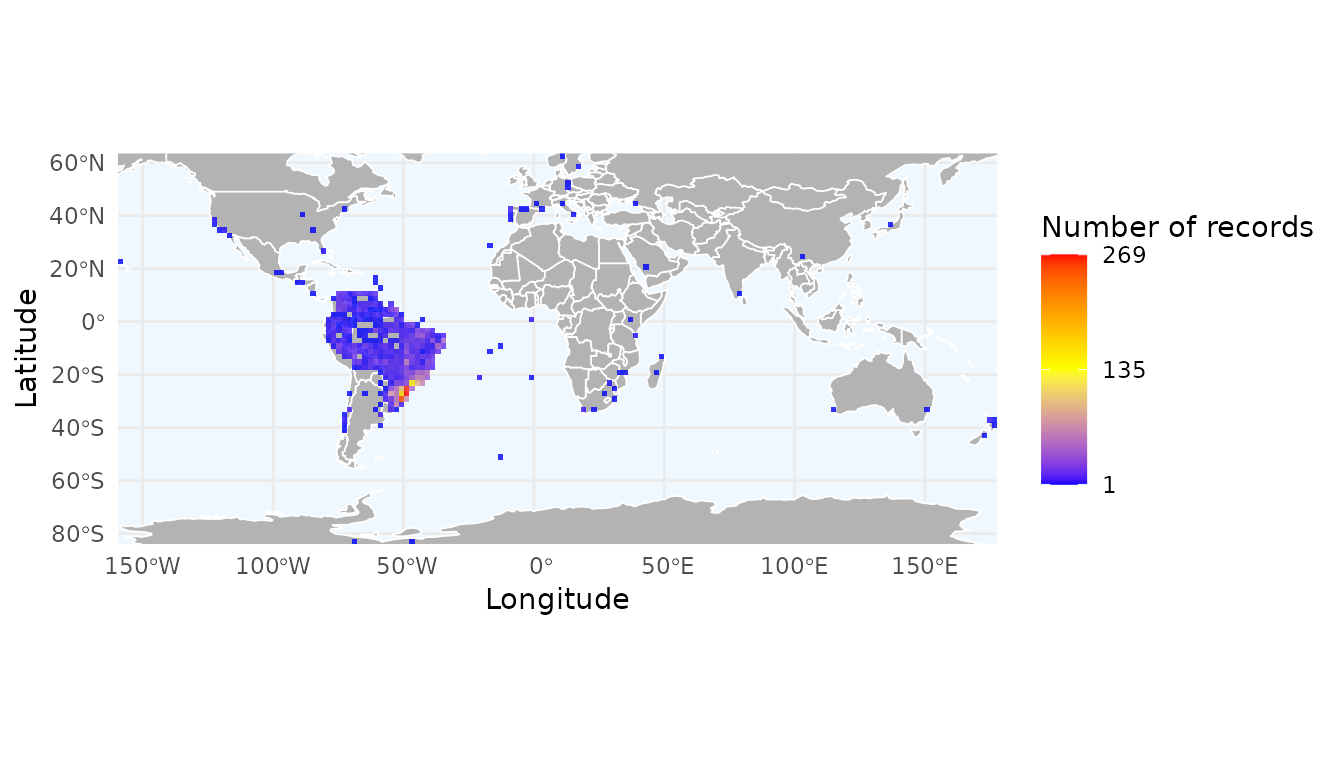
Mapping data quality flags
You can use the field argument to summarize specific
quality flags. In this example, we create a density map of records
flagged because they are cultivated. This helps identify if certain
regions have a higher prevalence of cultivated specimens.
# Converting flag columns to numeric for plotting
# We invert the logic so that errors (FALSE) become 1 and clean data (TRUE) become 0
occ$cultivated_flag_num <- as.numeric(!occ$cultivated_flag)

# Create the grid
r_flagged <- richness_here(occ,
                           summary = "records",
                           field = "cultivated_flag_num",
                           field_name = "Cultivated records",
                           fun = sum,
                           res = 2)

# Plot with ggrid_here
ggrid_here(r_flagged,
           low_color = "white",
           mid_color = "orange",
           high_color = "firebrick")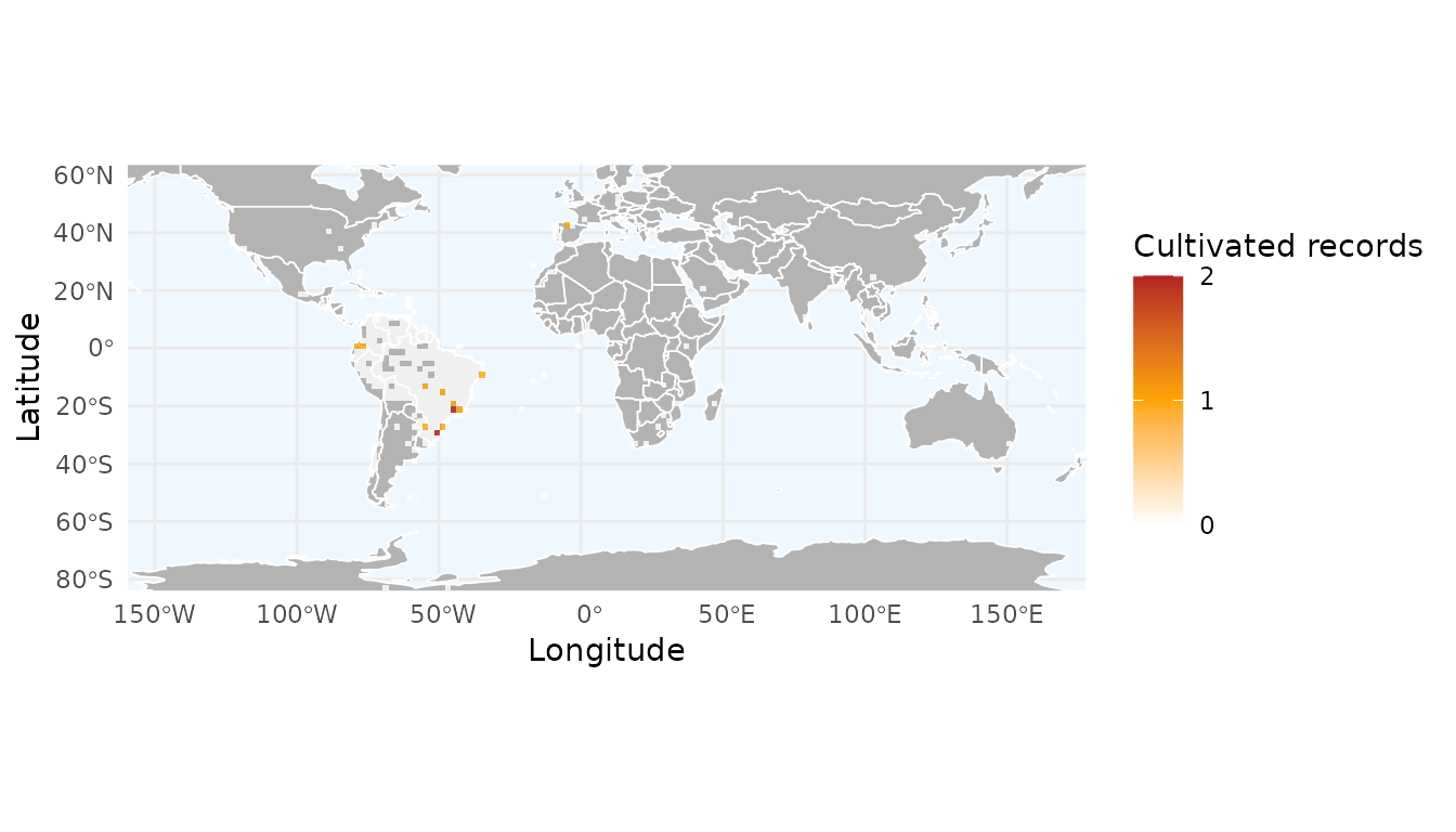
The field argument is highly flexible. While we used
flags here, you can replace the flag column with any numeric trait
(e.g., plant height, seed mass) or environmental variable. By changing
the fun argument to mean or median, you can easily generate maps of
average trait values across space.
In the next vignette, we demonstrate how to use expert-derived information from other biodiversity databases, such as the IUCN and the World Checklist of Vascular Plants, to identify records that fall outside the natural range of a species.