Introduction
For most studies relying on primary biodiversity data, sampling bias can be a problem because it creates clusters of points that reflect accessible areas and the preferences of the researchers who collected the data, rather than the ecological preferences of the species.
Two common approaches to mitigate sampling bias involve thinning
occurrence records (i.e., removing records that are close to each
other). Thinning can be performed in either geographic or environmental
space. The RuHere package allows the use of both approaches
and also enables combining the results of both methods.
As an example, let’s use the records of Araucaria angustifolia available in the package, after removing records flagged as potentially problematic:
# Load packages
library(RuHere)
library(terra)
#> terra 1.9.11
library(mapview)

# Import occurrence data
data("occ_flagged", package = "RuHere")
# Remove flagged records
occ <- remove_flagged(occ = occ_flagged)
# Plot records
ggmap_here(occ = occ)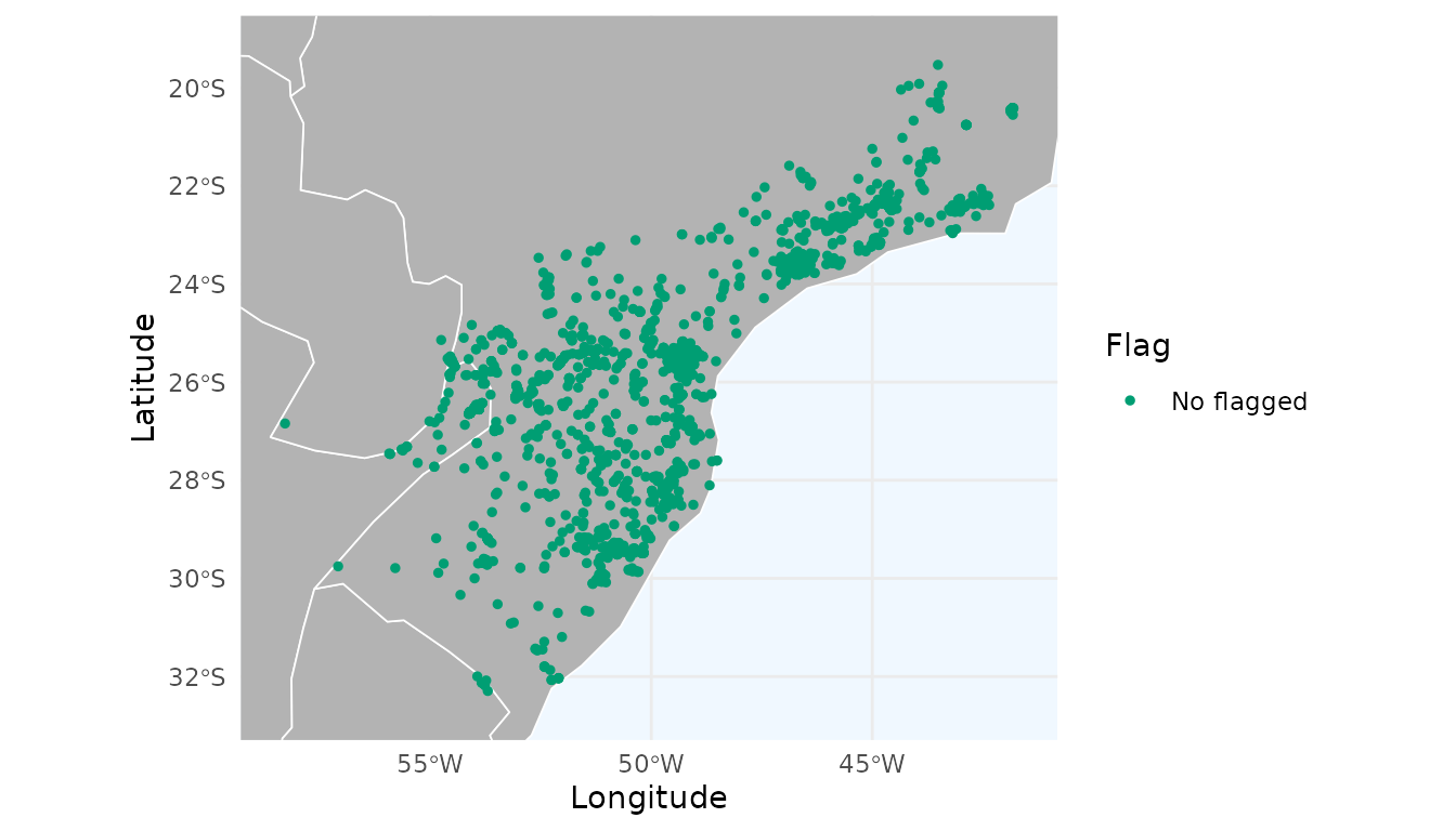
Heatmap for occurrence data
Before starting the thinning process, let’s create a heatmap based on a kernel density estimation of the records:
# Generate heatmap
heatmap <- spatial_kde(occ = occ, resolution = 0.2, buffer_extent = 50,
                       radius = 2, zero_as_NA = TRUE)
We can use the function ggmap_here() to plot the
occurrences and the heatmap (or use map_here() if you
prefer an interactive version).
ggmap_here(occ = occ, size_points = 0.5, heatmap = heatmap)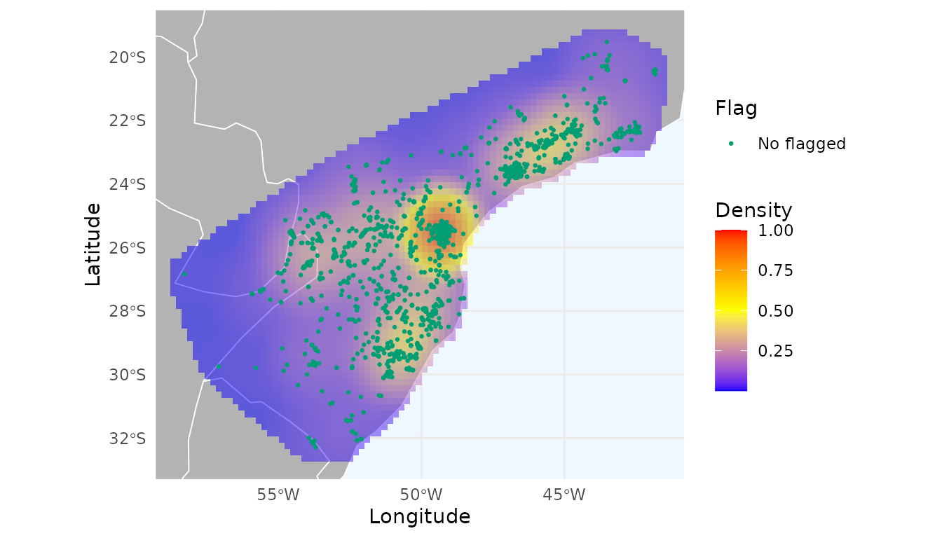
We can observe a notable hotspot with a cluster of records around Curitiba city (capital of Paraná, southern Brazil), which indicates strong sampling bias. Let’s evaluate the effect of thinning these records in geographic space.
Thinning in geographic space
The thin_geo() function flags occurrence records for
thinning by keeping only one record per species within a radius of
d kilometers. This function is similar to
thin() from the spThin
package, but with an important difference: it allows specifying a
priority order for retaining records.
When a thinning distance is provided (e.g., 10 km), the function
identifies clusters of records within that distance. Within each
cluster, it retains the record with the highest priority according to
the column defined in prioritary_column (for example, using the most
recent record when prioritary_column = "year"), and flags
all remaining nearby records for removal. If
prioritary_column is NULL, the priority
follows the original row order of the input occ data frame.
Let’s thin the records using a 10 km radius and keep the most recent record as the priority:
# Thin records using a 10 km distance threshold
occ_thin <- thin_geo(occ = occ, d = 10, prioritary_column = "year")
sum(!occ_thin$thin_geo_flag)  # Number of records flagged for removal
#> [1] 1860
The function flagged 1,860 records for removal. Let’s visualize the
flagged records using map_here() and create a heatmap with
the remaining records.
# Remove flagged records
occ_thin_geo <- remove_flagged(occ = occ_thin)
# Create heatmap
heatmap_thin_geo <- spatial_kde(occ = occ_thin_geo, resolution = 0.2,
                                buffer_extent = 50, radius = 2,
                                zero_as_NA = TRUE)
# Plot
ggmap_here(occ_thin, size_points = 0.5, heatmap = heatmap_thin_geo)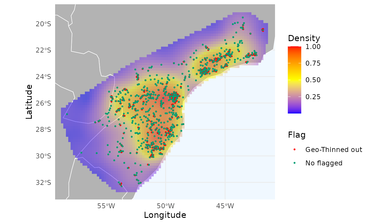
The thinned dataset (in green) produces a more spatially uniform heatmap and reduces the strong sampling bias around Curitiba. We explore different distance thresholds in the next section.
Selecting the best distance to thin records
A key question is determining the optimal thinning distance, since we rarely have sufficient biological justification for choosing a specific value. To address this issue, we adapted the approach of Velazco et al. (2020), which computes spatial autocorrelation (Moran’s I) for datasets generated using different thinning distances and selects the distance that yields the lowest average spatial autocorrelation.
We extended this procedure by adjusting the selection rules to avoid
choosing datasets with too few records or unrealistically low Moran’s I
values. See help(flag_geo_moran) for full details of the
selection procedure.
As an example, let’s test the effect of thinning using distances of 1, 3, 5, 7, 10, 15, 20, and 30 km. For computing spatial correlation, we need a raster containing the environmental variables. Here, we again specify a priority for retaining records (the most recent ones).
# Load example of raster variables
data("worldclim", package = "RuHere")
# Unwrap Packed raster
r <- terra::unwrap(worldclim)
# Select thinned occurrences
occ_geo_moran <- flag_geo_moran(occ = occ,
                                d = c(1, 3, 5, 7, 10, 15, 20, 30),
                                prioritary_column = "year",
                                env_layers = r)
#> Filtering records...
#> Calculating spatial autocorrelation using Moran Index...
The results for each tested distance are returned in the
imoran data.frame. It includes Moran’s I for each variable
and summary statistics across variables (mean, median, minimum, and
maximum), along with the number of retained records
(n_filtered) and the proportion of records flagged
(prop_lost).
occ_geo_moran$imoran
#>                   species Distance      bio_1     bio_7    bio_12 median_moran
#> 1  Araucaria angustifolia        1 0.26797715 0.4154464 0.2700062    0.2700062
#> 3  Araucaria angustifolia        3 0.20037829 0.3587940 0.1982657    0.2003783
#> 5  Araucaria angustifolia        5 0.17522297 0.3368257 0.1765754    0.1765754
#> 7  Araucaria angustifolia        7 0.16065669 0.3235316 0.1695589    0.1695589
#> 10 Araucaria angustifolia       10 0.15567148 0.2954804 0.1622244    0.1622244
#> 15 Araucaria angustifolia       15 0.14275985 0.2697169 0.1536365    0.1536365
#> 20 Araucaria angustifolia       20 0.13085143 0.2802101 0.1463788    0.1463788
#> 30 Araucaria angustifolia       30 0.09891003 0.2382515 0.1634006    0.1634006
#>    mean_moran  min_moran max_moran n_filtered all_records prop_lost
#> 1   0.3178099 0.26797715 0.4154464       1236        2426 0.4905194
#> 3   0.2524793 0.19826573 0.3587940        878        2426 0.6380874
#> 5   0.2295414 0.17522297 0.3368257        732        2426 0.6982688
#> 7   0.2179157 0.16065669 0.3235316        634        2426 0.7386645
#> 10  0.2044587 0.15567148 0.2954804        517        2426 0.7868920
#> 15  0.1887044 0.14275985 0.2697169        386        2426 0.8408904
#> 20  0.1858135 0.13085143 0.2802101        313        2426 0.8709810
#> 30  0.1668540 0.09891003 0.2382515        206        2426 0.9150866
The “best” distance that reduces the spatial autocorrelation without discarding too many records was 15km. Using this threshold, 2,040 records were flagged.
# Best distance selected
occ_geo_moran$distance
#> [1] "15"
# Number of flagged records using this distance to thin
sum(!occ_geo_moran$occ$thin_geo_flag)
#> [1] 2040
Visual inspection shows an even more uniform heatmap:
# Remove flagged records
occ_thin_geo_moran <- remove_flagged(occ = occ_geo_moran$occ)
# Create heatmap
heatmap_thin_geo_moran <- spatial_kde(occ = occ_thin_geo_moran,
                                      resolution = 0.2,
                                      buffer_extent = 50, radius = 2,
                                      zero_as_NA = TRUE)
ggmap_here(occ = occ_geo_moran$occ, size_points = 0.5,
           heatmap = heatmap_thin_geo_moran)
A potential issue when filtering records in geographic space is that
two nearby records may actually occur in distinct environmental
conditions, especially in highly heterogeneous regions. This can lead to
the loss of unique information about the species’ niche and
environmental tolerances. To address this, we can instead apply thinning
in environmental space, as explored in the next sections.
Thinning in environmental space
Thinning in environmental space removes records with similar
environmental conditions, representing redundant ecological information.
This is achieved by building a multidimensional grid in environmental
space, dividing each variable into n_bins equally sized
intervals. Each record is assigned to a unique environmental block (a
combination of bins), and records within the same block (i.e.,
environmentally similar) are flagged for removal.
To illustrate how the environmental grid works, let’s use
get_env_bins() with 10 bins:
# Get bins
b <- get_env_bins(occ = occ, env_layers = r, n_bins = 10)
head(b$data)
#>      bio_1  bio_7 bio_12 bio_1_bin bio_7_bin bio_12_bin block_id
#> 1 17.69396 18.667   1523         5         5          3    5_5_3
#> 2 17.10746 17.701   1397         5         4          2    5_4_2
#> 3 16.44496 19.445   1698         4         6          4    4_6_4
#> 4 18.17946 22.320   1872         6         9          5    6_9_5
#> 5 19.71071 18.632   1496         7         5          3    7_5_3
#> 6 17.77913 19.411   1576         5         6          3    5_6_3
The function returns the environmental block IDs for each record. We can visualize the grid for any two variables:
# Plot
plot_env_bins(b, x_var = "bio_1", y_var = "bio_12",
              xlab = "Temperature", ylab = "Precipitation")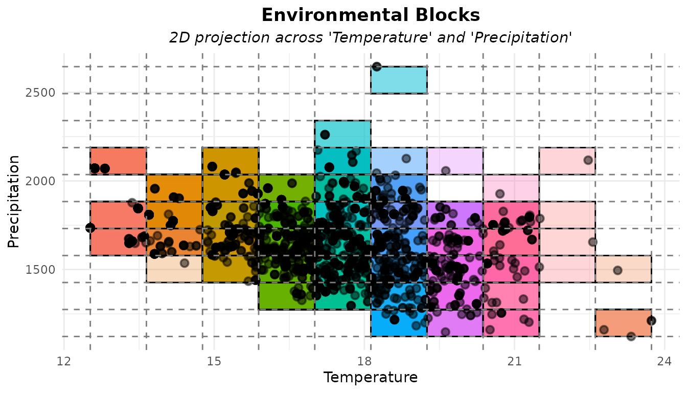
We can see that several records fall into the same block, meaning
they are environmentally similar and therefore redundant. Let’s flag
these redundant records using thin_env():
# Flag records that are close to each other in the enviromnetal space
occ_thin_env <- thin_env(occ = occ, env_layers = r, n_bins = 10,
                         prioritary_column = "year")
# Number of flagged (redundant) records
sum(!occ_thin_env$thin_env_flag) #Number of flagged records
#> [1] 2227
The function flagged 2,227 records. Let’s visualize these and create a heatmap of the remaining data.
# Remove flagged records
occ_thinned_env <- remove_flagged(occ = occ_thin_env)
# Create heatmap
heatmap_thin_env <- spatial_kde(occ = occ_thinned_env, resolution = 0.2,
                                buffer_extent = 50, radius = 2,
                                zero_as_NA = TRUE)
ggmap_here(occ_thin_env, size_points = 0.5, heatmap = heatmap_thin_env)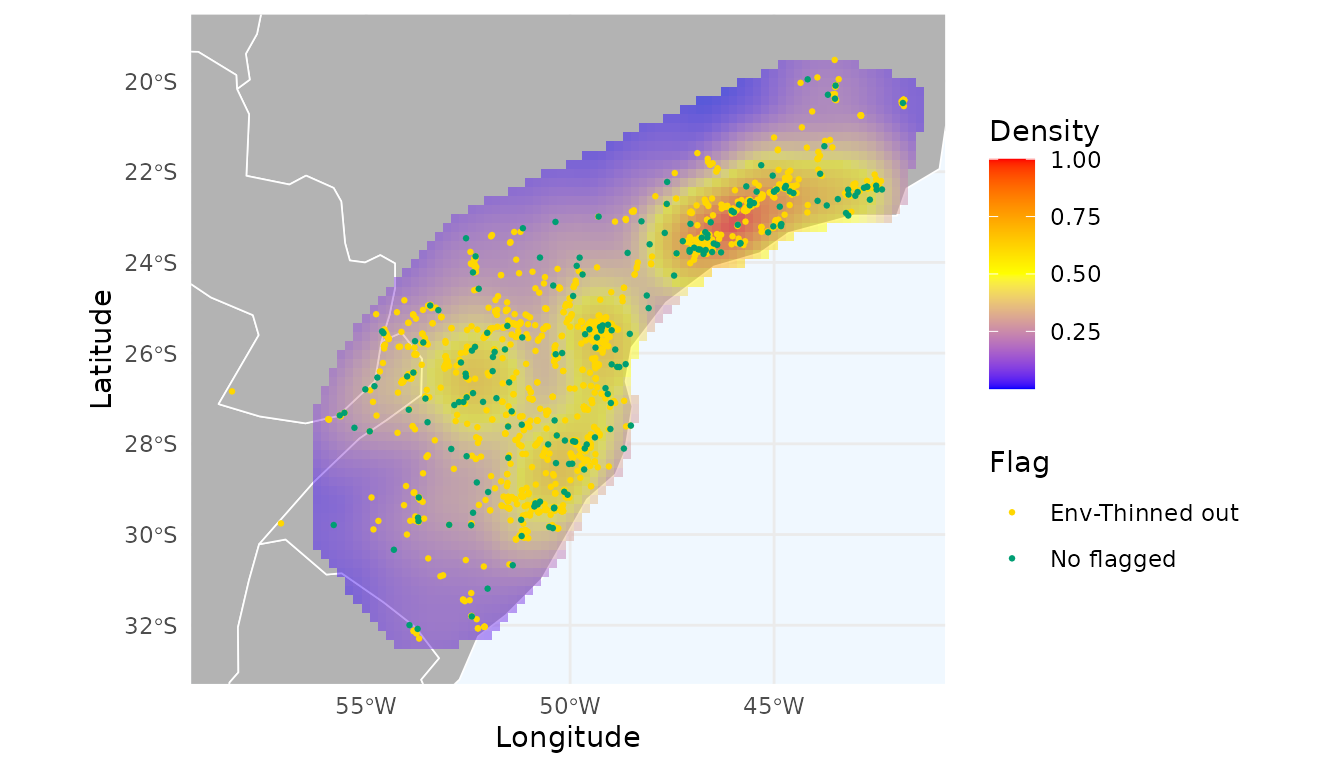
Thinning in environmental space produces a spatial pattern that differs from the dataset filtered exclusively in geographic space.
Similar to the thinning process in geographic space, we can test different numbers of bins (see next section).
Selecting the best number of environmental bins
In geographic thinning, the key parameter is distance. In environmental thinning, it is the number of bins. More bins result in finer partitions of environmental space, reducing the chances of records falling into the same block. As with geographic thinning, we can test multiple bin values and select the one that reduces spatial autocorrelation without discarding many records.
Here, we test 5, 10, 20, 30, 40, 50, 60, 70, and 80 bins:
# Select thinned occurrences
occ_env_moran <- flag_env_moran(occ = occ,
                                n_bins = c(5, 10, 20, 30, 40, 50, 60, 70, 80),
                                prioritary_column = "year",
                                env_layers = r)
#> Filtering records...
#> Calculating spatial autocorrelation using Moran Index...
Again, results are returned in an imoran data frame. It includes
Moran’s I for each variable and summary statistics across variables
(mean, median, minimum, and maximum), along with the number of retained
records (n_filtered) and the proportion of records flagged
(prop_lost).
occ_env_moran$imoran
#>                   species n_bins     bio_1     bio_7    bio_12 median_moran
#> 5  Araucaria angustifolia      5 0.2401256 0.3282298 0.1749087    0.2401256
#> 10 Araucaria angustifolia     10 0.2099819 0.3770858 0.1764008    0.2099819
#> 20 Araucaria angustifolia     20 0.1762887 0.3638996 0.1923568    0.1923568
#> 30 Araucaria angustifolia     30 0.1787372 0.3657022 0.1944775    0.1944775
#> 40 Araucaria angustifolia     40 0.1903925 0.3540410 0.1927357    0.1927357
#> 50 Araucaria angustifolia     50 0.1873899 0.3515700 0.1926828    0.1926828
#> 60 Araucaria angustifolia     60 0.1839720 0.3525726 0.1930614    0.1930614
#> 70 Araucaria angustifolia     70 0.1839973 0.3561391 0.1930398    0.1930398
#> 80 Araucaria angustifolia     80 0.1865604 0.3558738 0.1934019    0.1934019
#>    mean_moran min_moran max_moran n_filtered all_records prop_lost
#> 5   0.2477547 0.1749087 0.3282298         57        2426 0.9765045
#> 10  0.2544895 0.1764008 0.3770858        199        2426 0.9179720
#> 20  0.2441817 0.1762887 0.3638996        504        2426 0.7922506
#> 30  0.2463056 0.1787372 0.3657022        658        2426 0.7287716
#> 40  0.2457231 0.1903925 0.3540410        715        2426 0.7052762
#> 50  0.2438809 0.1873899 0.3515700        748        2426 0.6916735
#> 60  0.2432020 0.1839720 0.3525726        757        2426 0.6879637
#> 70  0.2443921 0.1839973 0.3561391        767        2426 0.6838417
#> 80  0.2452787 0.1865604 0.3558738        769        2426 0.6830173
The “best” number of bins that reduces the spatial autocorrelation without discarding too many records was 70. With this threshold, 1,659 records were flagged.
# Best distance selected
occ_env_moran$n_bins
#> [1] "70"
# Number of flagged records using this distance to thin
sum(!occ_env_moran$occ$thin_env_flag)
#> [1] 1659
Let’s check the distribution of these records and the heatmap generated with the unflagged records:
# Remove flagged records
occ_thin_env_moran <- remove_flagged(occ = occ_env_moran$occ)
# Create heatmap
heatmap_thin_env_moran <- spatial_kde(occ = occ_thin_env_moran,
                                      resolution = 0.2,
                                      buffer_extent = 50, radius = 2,
                                      zero_as_NA = TRUE)
ggmap_here(occ = occ_env_moran$occ, size_points = 0.5,
           heatmap = heatmap_thin_env_moran)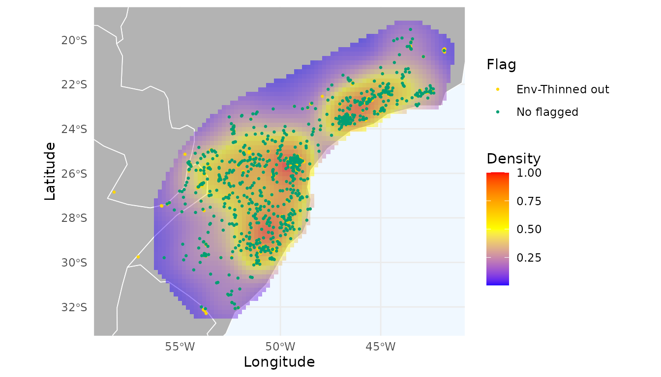
Consensus between environmental and geographic thinning
Thinning in environmental space can suffer from the opposite issue of geographic thinning: environmentally similar records may be geographically far apart, potentially removing important information about the species’ geographic range.
To address this, the flag_consensus() function can be
used to flag records only when they are redundant in both geographic and
environmental space.
# Flag occurrences by thinning in geographic space
occ_geo_moran <- flag_geo_moran(occ = occ,
                                d = c(1, 3, 5, 7, 10, 15, 20, 30),
                                prioritary_column = "year",
                                env_layers = r)
#> Filtering records...
#> Calculating spatial autocorrelation using Moran Index...

# Flag occurrences by thinning in environmental space
occ_env_moran <- flag_env_moran(occ = occ_geo_moran$occ,
                                n_bins = c(5, 10, 20, 30, 40, 50, 60, 70, 80),
                                prioritary_column = "year",
                                env_layers = r)
#> Filtering records...
#> Calculating spatial autocorrelation using Moran Index...
# Get consensus
occ_consensus <- flag_consensus(occ = occ_env_moran$occ,
                                flags = c("thin_geo", "thin_env"),
                                consensus_rule = "any_true",
                                flag_name = "thin_geo_env_flag")
# Remove flagged
occ_consensus_filtered <- remove_flagged(occ = occ_consensus, flags = NULL,
                                         additional_flags = c("thin_geo_env" = "thin_geo_env_flag"))

# Create heatmap
heatmap_consensus_filtered <- spatial_kde(occ = occ_consensus_filtered,
                                          resolution = 0.2,
                                          buffer_extent = 50,
                                          radius = 2, zero_as_NA = TRUE)
Let’s visualize which records were flagged by geographic thinning, environmental thinning, or both:
ggmap_here(occ = occ_consensus,
          flags = c("thin_geo", "thin_env"),
          additional_flags = "thin_geo_env_flag",
          names_additional_flags = "Thinned geo-env",
          col_additional_flags = "blue",
          size_points = 0.5,
          heatmap = heatmap_consensus_filtered)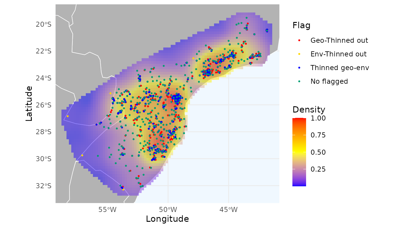
Red points indicate records thinned in geographic space; yellow points indicate thinning in environmental space; and blue points indicate records thinned in both.
Note that we retained the records flagged only in the geographic thinning, those flagged only in the environmental thinning, and those not flagged by either method.