3. Using faunabr to flag erroneous records
Source:vignettes/Spatialize_faunabr.Rmd
Spatialize_faunabr.RmdLoading data
Before you begin, use the load_faunabr function to load
the data. For more detailed information on obtaining and loading the
data, please refer to 1. Getting started
with faunabr
library(terra)
#Load data
bf <- load_faunabr(data_dir = my_dir, #Folder where you stored the data with the function get_faunabr()
                   data_version = "latest",
                   type = "short") #short version
#> Loading version 1.3
Get spatial polygons of species distribution
Fauna do Brasil provides information on the brazilian federal states
and countries with confirmed occurrences of the species. The
get_spat_occ function extracts these information and return
Spatial polygons (SpatVectors) representing the distribution of the
specie. We can choose getting the Spatialvector of the brazilian federal
states and/or countries.
#Example species
spp <- c("Panthera onca", "Mazama jucunda")
#Get spatial polygons
spp_spt <- fauna_spat_occ(data = bf, species = spp, state = TRUE,
                          country = TRUE, verbose = TRUE)
#> Getting states of Panthera onca
#> Getting countries of Panthera onca
#> Getting states of Mazama jucunda
#> Getting countries of Mazama jucunda
The SpatVectors are stored in a nested list by species:
par(mfrow = c(3, 2), mar = c(2, 0, 2, 0))
plot(spp_spt$`Panthera onca`$states,
     main = paste0(names(spp_spt)[[1]], " - States"), mar = NA)
plot(spp_spt$`Panthera onca`$countries,
     main = paste0(names(spp_spt)[[1]], " - Countries"), mar = NA)
plot(spp_spt$`Mazama jucunda`$states,
     main = paste0(names(spp_spt)[[2]], " - States"), mar = NA)
plot(spp_spt$`Mazama jucunda`$countries,
     main = paste0(names(spp_spt)[[2]], " - Countries"), mar = NA)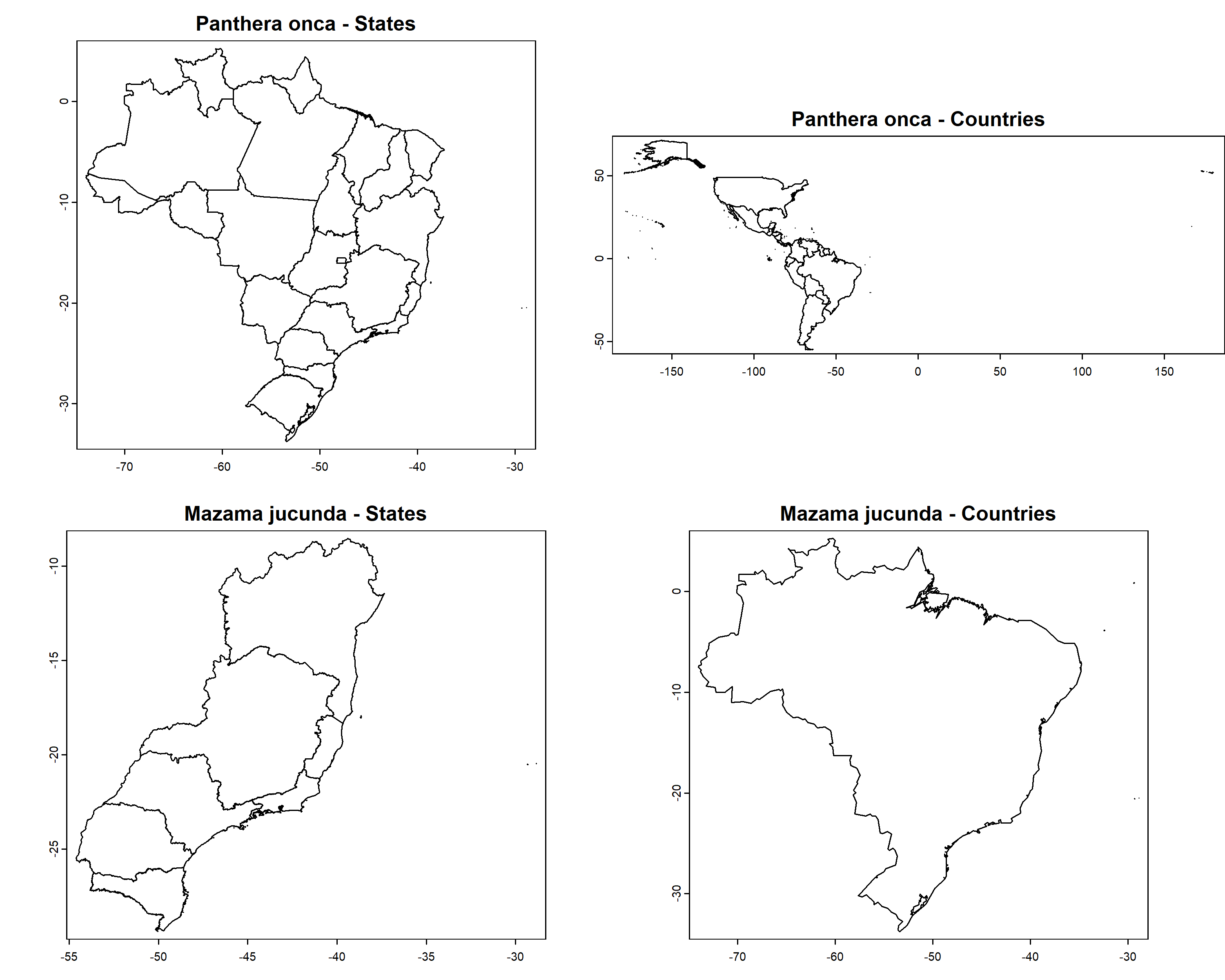
Filtering occurrence records using distribution information in Fauna do Brasil
Georeferencing errors in online species records can introduce
significant bias into ecological and biogeographical research findings.
Some R packages, as CoordinateCleaner,
help to flagging common spatial errors in biological collection data,
for example, records of terrestrial organism that fall in the sea or
were assigned to capital and province centroids. Since the distributions
of species in Fauna do Brasil are based on the expertise of taxonomists,
it represents a valuable information to add an additional step on
checking the validity of occurrence records got from online databases
(as GBIF or SpeciesLink). The filter_faunabr function
automatized this flagging. You can use the function to flag and/or
remove records that fall outside the brazilian states or countries with
confirmed occurrence according to Fauna do Brasil.
As example, let’s use the occurrence records of two species.
Panthera onca is a terrestiral felidae with confirmed
occurrences in 22 of the 27 brazilian states (absent in Rio Grande do
Norte, Paraíba, Pernambuco, Alagoas, and Sergipe) and 20 countries.
Chaetomys subspinosus is an arboreal rodent endemic to Brazil
with confirmed occurrences in 5 states (Bahia, Espírito Santo, Minas
Gerais, Rio de Janeiro, and Sergipe). Let’s plot these information using
the function get_spat_occ:
my_spp <- c("Panthera onca", "Chaetomys subspinosus")
pol_spp <- fauna_spat_occ(data = bf, species = my_spp,
state = TRUE, country = TRUE,
verbose = TRUE)
par(mfrow = c(2, 2), mar = c(2, 0, 2, 0))
plot(pol_spp$`Panthera onca`$states,
main = paste0(names(pol_spp)[[1]], " - States"), mar = NA)
plot(pol_spp$`Panthera onca`$countries,
main = paste0(names(pol_spp)[[1]], " - Countries"), mar = NA)
plot(pol_spp$`Chaetomys subspinosus`$states,
main = paste0(names(pol_spp)[[2]], " - States"), mar = NA)
plot(pol_spp$`Chaetomys subspinosus`$countries,
main = paste0(names(pol_spp)[[2]], " - Countries"), mar = NA)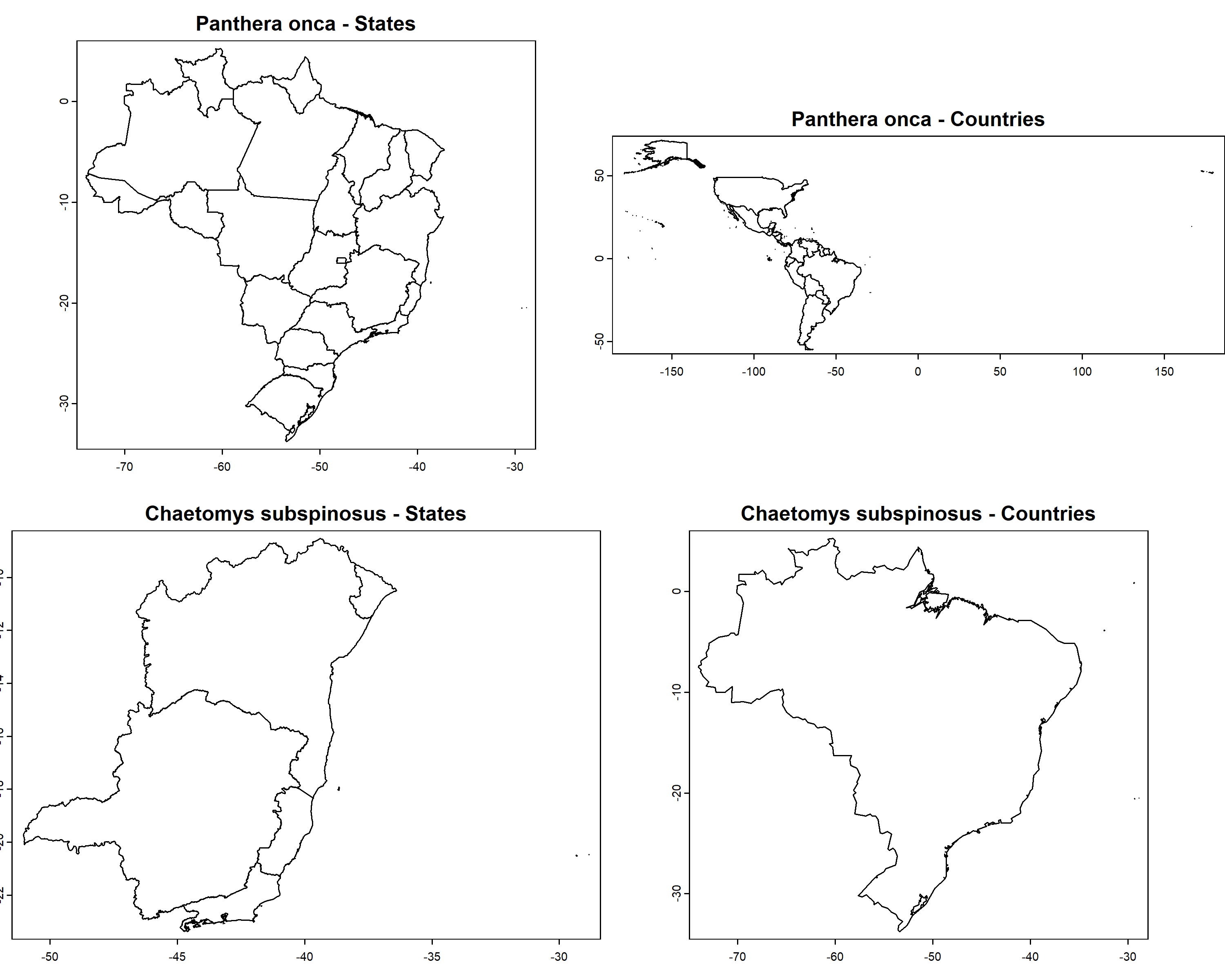 We downloaded the
occurrences of these two species from GBIF using the
We downloaded the
occurrences of these two species from GBIF using the
plantR::rgbif2() function. These occurrences are saved as
data examples in the package and we can import it:
data("occurrences")
head(occurrences)
#>         species         x          y  source
#> 1 Panthera onca -90.38409  17.377023    gbif
#> 2 Panthera onca -90.24368  17.240507    gbif
#> 3 Panthera onca -77.36680   0.287624    gbif
#> 4 Panthera onca -56.61023 -17.239688    gbif
#> 5 Panthera onca -61.04386  -2.387029    gbif
#> 6 Panthera onca -77.28850   0.288757    gbif
The input data with records must be a dataframe with at least 3 columns: one informing the species name, one informing the longitude and one informing the latitude. Let’s check if there are records outside of the species’ natural ranges considering states and countries:
occ_check <- filter_faunabr(data = bf, occ = occurrences,
                    by_state = TRUE, buffer_state = 20,
                    by_country = TRUE, buffer_country = 20,
                    value = "flag&clean", keep_columns = TRUE,
                    verbose = FALSE)
#> Returning list with flagged and cleaned occurrences
Since we set value = “flag&clean”, the function returned a list with two data.frames: one with all the records flagged if on each test they passed (TRUE) or not (FALSE); and another with only the records that passed in all tests.
Let’s use the mapview package to plot an interactive map of the flagged records:
#Install mapview if necessary and load package
if(!require(mapview)){
    install.packages("mapview")
}
#Load mapview
library(mapview)
Let’s check the records of Panthera onca, plotting the records and the map got previously. You can see that the green records passed on the test of States, falling in the states with confirmed occurrence of the specie. The red dots are the records that falls outside the states. The gray dots are records that was not testes because they falls outside Brazil.
#Convert points to spatvector
panthera_occ <- subset(occ_check$flagged,
occ_check$flagged$species == "Panthera onca")
panthera_occ <- vect(panthera_occ, geom = c("x", "y"),
crs = crs(pol_spp$`Panthera onca`$states))
#Iteractive plot
mapview(pol_spp$`Panthera onca`$states,
layer.name = "States with confirmed occurrences") +
mapview(panthera_occ, zcol = "inside_state", layer.name = "Inside state?",
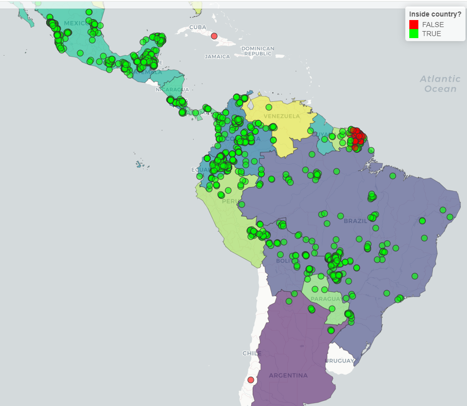
col.regions = c("red", "green"))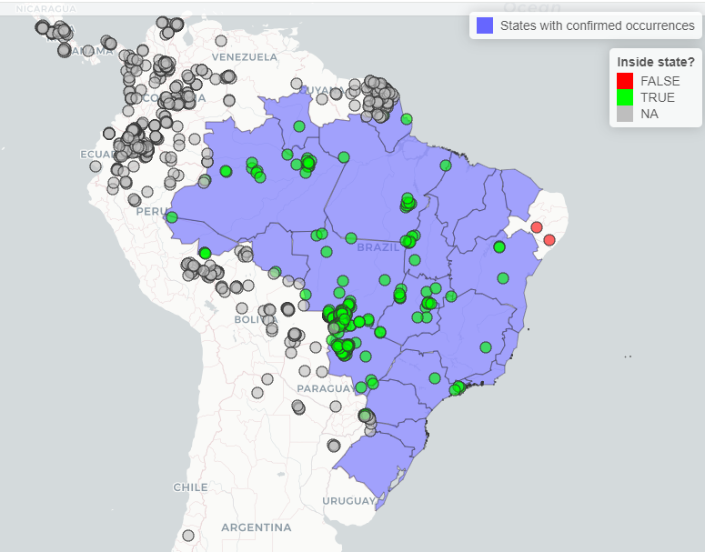 We can see the same with countries: green dots represents records that
passed in the test and green dots represents records that did not passed
the test.
We can see the same with countries: green dots represents records that
passed in the test and green dots represents records that did not passed
the test.
#Iteractive plot
mapview(pol_spp$`Panthera onca`$countries,
        layer.name = "Countries with confirmed occurrences", burst = TRUE, legend = F) +
  mapview(panthera_occ, zcol = "inside_country",
          col.regions = c("red", "green"),
          layer.name = "Inside country?")